My firm is frequently engaged by companies to analyze data. One example is a manufacturer of building materials. The company’s profit was stagnant. It asked us to analyze sales data for customers, products, and regions to determine where to focus its marketing efforts and where to streamline operations, to lower costs.
In this post, I’ll describe that engagement and its findings.
Preparing the Data
The purpose of the engagement was simple: to determine ways to increase profit. To do this, we analyzed sales data, including:
- Date of sale,
- Customer name or number,
- Destination city and state,
- SKU or simple product description,
- Warehouse where the SKU is stored.
The client provided 10 years of data to enable us to review trends.
The first step was to prepare the data — i.e., organize the segments. This is typically done in a spreadsheet such as Excel. For the building materials engagement, our process included:
- Categorize SKUs by material, design, and type. Some products had more than 10 such attributes.
- Categorize customers by type. For example, business customers could be small independent retailers or a big box stores. For consumer buyers, we captured household and demographic info, including gender (from the name).
- Categorize ship-to location. Was the destination urban or rural? Did customers live in condos and townhouses in urban areas or in detached homes in suburban or rural areas?
Running the Analysis
The second step was to run the analysis using various analytical models, including cluster analysis, segmentation analysis, decision tree modeling, and simple descriptive analytics. You can use statistical software such as SPSS Statistics or SAS, or programming languages such as R or Python.
- Cluster analysis is the statistical technique of grouping products by attributes, such as products that are closest in profit margins or are popular in certain regions.
- Segmentation analysis groups customers or products by type. For example, one customer segment could be independent contractors. Another could be interior designers. Product types could be items for commercial buildings versus residences. You could also group customers geographically, perhaps urban versus rural.
- Decision tree modeling is a way to split the data into different subsets. It typically starts with binary splits and continues until there is nothing to split. For example, if you set a decision tree to identify customers with the most sales, you can use it to identify the types of products with the most sales, too.

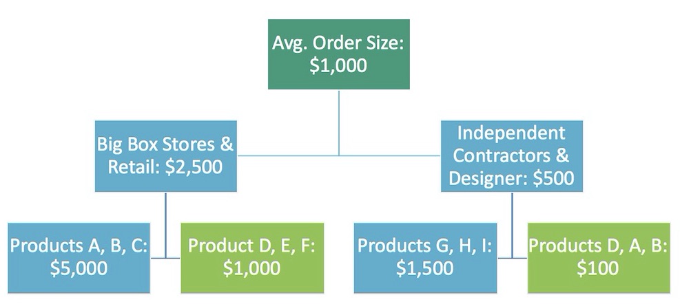
This hypothetical decision tree shows the split between customer types and the products ordered with the average size. Big box and retail stores have a higher order size ($2,500) especially for products A, B, C ($5,000). Independent contractors and designers have a lower average order size ($500), especially for products D, A, B ($100).
- Descriptive analytics is a simple approach to summarizing historical data by asking questions. Examples include “What is the average order size?” and “Which type of customers (contractors or big box stores) purchase the most dollar volume?” Descriptive analysis is the first step in modeling to see if there is a difference between customers or products.
Reviewing the Findings
Our analysis produced the following findings.
- Profitable products. Twenty percent of SKUs collectively contributed less than 1 percent of total sales. Therefore, ceasing the manufacturing of those SKUs would greatly increase profit.
- Big box stores purchased a relatively limited number of SKUs, which they ordered in bulk. Big box stores did not purchase new products. This led to an internal discussion as to the reasons. Possibilities included (a) a lack of marketing support for new product launches, (b) the need to test new products before nationwide rollouts, and (c) the prices of new products.
- Independent contractors were a hidden gem, which was unexpected. While the quantities were small, they typically ordered higher-margin products. Moreover, independent contractors held much growth potential. Therefore, the company shifted marketing efforts to this segment of customers.
- Interior designers represented less than 0.01 percent of overall sales. However, interior designers frequently ordered the new products and in certain regions impacted trends.
- Geographic influences. There was a clear distinction among geographic markets. Home interiors differed by region, for example. Consumers in California purchased different products, materials, and colors than consumers in Ohio.
The Surprise
Combining sales and warehouse data uncovered a surprise. The company had four warehouses. Each stored roughly the same SKUs at similar quantities.
Adding geographical preferences to bulk orders from the big box stores and removing products that were not selling enabled the company to save money. While the logistics department was optimizing transit times, no one thought to look at the sales from each warehouse. But looking at geographic preferences, we identified SKUs that are needed for each region and each warehouse, thereby cutting distribution and storage costs.


