Using COUNTIF, COUNTIFS in Google Sheets to Sort, Analyze Data

Whether you’re researching keywords, reviewing lead sources, or analyzing customer attributes from a CRM export, Google Sheets’ COUNTIF and COUNTIFS formulas can help.

These two spreadsheet formulas will only count a cell (from a range of cells) if specific criteria are met.

Recently, a multichannel retailer wanted to analyze five years’ worth of lead and conversion data from its customer relationship management software. Leads might come from the retailer’s website, its various digital marketing efforts, offline advertising, or folks just walking into a store.

…a multichannel retailer wanted to analyze five years’ worth of lead and conversion data…

The company sells relatively expensive products that range from $10,000 to $50,000 each. Thus, it may take a few contacts to close a sale. Understanding which sources produce leads could help the retailer understand how to get more customers.

Unfortunately, the company’s CRM did not provide the required report. So a couple of folks from the retailer’s marketing department exported the data in comma-separated values format. This CSV file was uploaded to a Google Sheet, and thanks to COUNTIF and COUNTIFS, it was fairly easy to identify which lead sources produced the most sales.

To demonstrate how to apply COUNTIF and COUNTIFS formulas, I’ll use sample data.

COUNTIF

The data has four columns: an order number, the U.S. state from which the order was placed, the lead source, and the sale amount. For the examples, I’ll focus on just two of these columns: the state and the lead source. The name of the sheet is “Lead Data.” Notice that I included this name the range of cells.

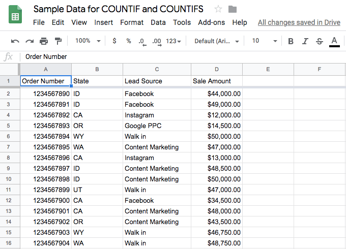
The example or sample data as it appeared in a Google Sheet. Notice the four columns of data; our examples will focus on state and lead source. Click image to enlarge.

I will create a second sheet to analyze lead sources by U.S. state. This sheet will have a column to list the states, the total count for each state, and the count and percentage of the total for each lead source.

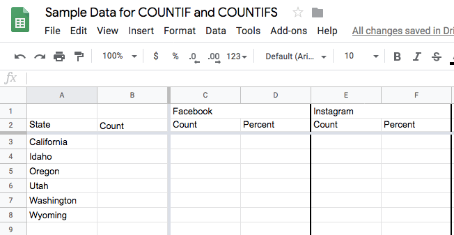
A second sheet will employ the COUNTIF and COUNTIFS formulas. It includes a pair of columns — “Count” and “Percent” —  for each lead source. Each state’s count is in a row. Click image to enlarge.

I will use the COUNTIF formula to get the total number of orders originating from each state. The formula accepts two parameters, the range and the criterion.

=COUNTIF(range, criterion)

The range is any set of cells in the current sheet or another sheet. Our range will come from the “Lead Data” sheet and not the current one.

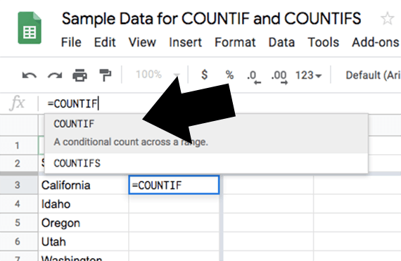
Typing  “=COUNTIF” into the formula bar in Google Sheets will auto-generate formula options from a list. Select “=COUNTIF” and navigate to the range and then drag to select it.

Google Sheets will recognize the COUNTIF formula as you start to type it. Click image to enlarge.

When a cell contains text, the criterion is quoted. For our example, I first wanted to get a count of all of the sales to California — designated as “CA” in the cells of the state column. This is what the COUNTIF formula looked like:

=COUNTIF('Lead Data' !B2:B25, "CA")

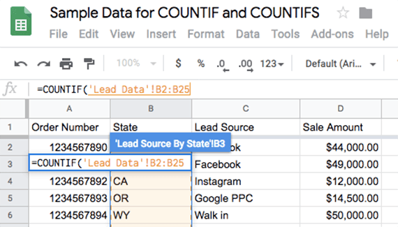
The range should appear as you select it in the Google Sheets’ formula bar. Then type a comma and the criterion value. Click image to enlarge.

The section describing the sheet and range uses ‘Lead Data’ !B2:B25 as the range and the state (“CA”) for the criterion. If the range had been in the same or current sheet, it would not have included the sheet name.

I can use this same approach to get the count for each state on the list.

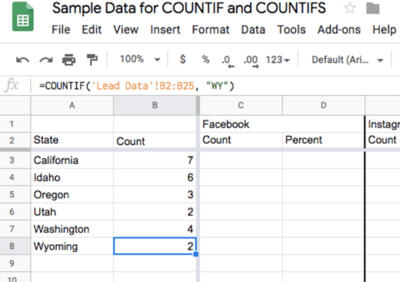
Use the COUNTIF formula to obtain a count for each of the states in consideration. Click image to enlarge.

COUNTIFS

The related COUNTIFS formula will accept a series of ranges and criterion pairs. We can use it to find the number of leads that converted from each source, such as Facebook.

The formula is similar to COUNTIF. In this case, we are counting only rows that have “CA” in the state column.

=COUNTIFS('Lead Data' !B2:B25, "CA")

To this, we add a comma, followed by a second range and a second criterion — Facebook in this example.

=COUNTIFS('Lead Data' !B2:B25, "CA", 'Lead Data' !C2:C25, "Facebook")

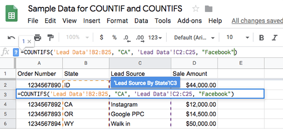
The COUNTIFS formula will allow for several series of range and criterion pairs separated by a comma. Click image to enlarge.

Changing the criterion for the state will give us a count of the leads from Facebook that converted consumers from each state. For our example, I also wanted to know the percentage of total leads these represented. So I can add a slash and a reference to the total leads for a given state.

=COUNTIFS(('Lead Data' !B2:B25, "CA", 'Lead Data'!C2:C25, "Facebook")/B3)

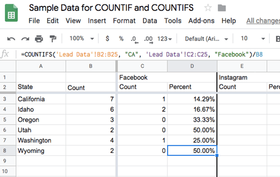
Use the COUNTIFS formula for each state and each lead source. The resulting count can be divided by the total number of converted leads for the state to get a percentage. Click image to enlarge.

Operators

You can also include operators in the criterion value for either COUNTIF or COUNTIFS. Place these inside the quotation marks surrounding the criterion value.

Here are some examples.

• “<>CA” — Not equal “CA” where “<>” means not equal.
• “>10” — Greater than 10.
• “<10” — Less than 10.
• “>=10” — Greater than or equal to 10.
• “<=10” — Less than or equal to 10.

Wildcards

Finally, there are also two available wildcard characters for criterion values.

• ? — Matches any single character.
• * — Matches zero or more contiguous characters.

To match an actual ? or *, put a tilde (~) in front of it. For example, “~?” would match a question mark.