Google Sheets SUMIF and SUMIFS functions help analyze, organize, and sum data based on specific criteria.
These formulas total cell values when they meet the requirements you set.
I recently did this for an online business that wanted to dig deep into its traffic reports.
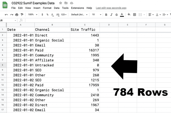
I exported the company’s daily site traffic by channel from its analytics software and imported that data into a Google Sheet, which I saved as “Daily Traffic.”
I then aggregated the data: one row per channel per day. The company receives traffic from roughly nine sources. Thus from January 1 to March 28 (87 days), the spreadsheet had 748 rows of channel-traffic totals. This was too much information to sort through manually.
Using sample data, let’s look at how the SUMIF and SUMIFS formulas can help analyze site traffic, specifically:
- How much traffic did each channel generate for the entire 87-day period?
- How much did each channel generate monthly?
SUMIF
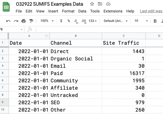
The imported traffic info has three columns: date, channel, and the number of unique visits for each channel on that day.
My first task is to figure out how much traffic each channel generated for the entire 87 days.
To begin, I created a sheet called “Total Traffic by Channel,” with two columns: “Channel” and “Total Traffic.”
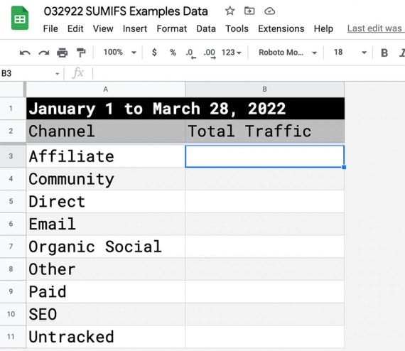
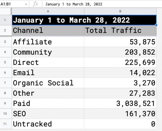
A new sheet, Total Traffic by Channel, contains the traffic totals for each channel for the entire period.
I used the SUMIF formula to obtain the total traffic from each channel for the entire date range. The formula accepts two or three parameters.
The two-parameter version includes “range” and “criterion.”
=SUMIF(range, criterion)
In this case, the range is where the formula will look for the criterion and the cells to sum.
For this example, we need the three-parameter version, which adds a “sum range.” That range is where Google Sheets will look when it matches the criterion. The sum range represents the cells to be totaled.
=SUMIF(range, criterion, sum range)
I’ll now use the formula to get the traffic from the affiliate channel.
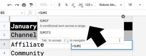
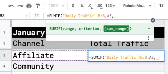
As I start to type “=SUMIF” into the formula bar, Google Sheets provides the option to select the SUMIF formula.
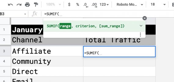
Because I selected the suggested SUMIF formula, Google Sheets showed me a guide. I can navigate around the workbook and select columns from the Daily Traffic sheet as needed.
I navigate to the “Daily Traffic” sheet and select column B.
Next, I need to define my criterion, which is the word “Affiliate.” Because I already have this word in my new sheet, Total Traffic by Channel, I can use the cell reference, A3.
Finally, I navigate back to the Daily Traffic sheet and select column C, the sum range. If Column B matches my criterion “Affiliate,” the value in Column C of the same row will be added to the total.
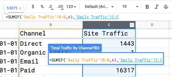
If Column B matches my criterion, “Affiliate,” the value in Column C of the same row will be added to the total.
Here is the completed formula.
=SUMIF('Daily Traffic'!B:B,A3,'Daily Traffic'!C:C)
Just like that, we know that the affiliate channel drove 53,875 site visits from January 1 through March 28.
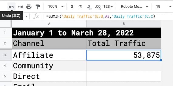
The SUMIF formula worked. The affiliate channel drove 53,875 visits from January 1 through March 28.
I can grab the bottom corner of this cell and drag the formula down to get the totals for each of the remaining channels.
The “Paid” (i.e., advertising) channel generated the lion’s share of traffic (3,038,521 visits), which is common for ecommerce sites.
SUMIFS
The SUMIFS function is similar to SUMIF, except it allows multiple criteria. This feature helps answer the second question, “How much traffic did each channel generate monthly?”
The parameters for SUMIFS are in a slightly different order.
=SUMIFS(sum range, criterion range, criterion)
It’s possible to have nearly unlimited criteria by adding pairs of criterion range and criterion.
=SUMIFS(sum range, criterion range 1, criterion 1, criterion range 2, criterion 2)
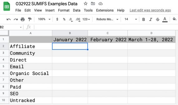
I’ve created another sheet, “Monthly Traffic by Channel,” with rows of channels and with columns of months.
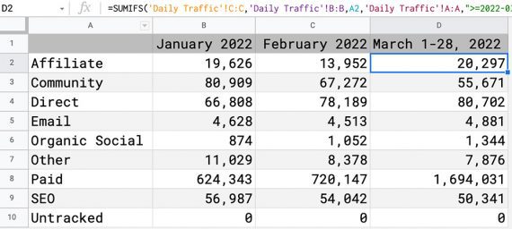
I’ve worked through the SUMIFS function in the same manner as the SUMIF function. Because it can include many criteria, the SUMIFs formula can get long. Eventually, I have the completed formula for the affiliate channel in January 2022.
=SUMIFS('Daily Traffic'!C:C,'Daily Traffic'!B:B,A2,'Daily Traffic'!A:A,">=2022-01-01",'Daily Traffic'!A:A,"<=2022-01-31")
Let’s break down this formula.
The first parameter is the sum range, column C in the Daily Traffic sheet. It contains the actual traffic volume.
=SUMIFS('Daily Traffic'!C:C,
The next two comma-separated parameters are the first criterion range and the first criterion.
'Daily Traffic'!B:B,A2
Column B in the Daily Traffic sheet (‘Daily Traffic’!B:B in the formula) is the list of channels. Cell A2 holds the channel name “Affiliate.” I could have typed “affiliate,” but using the cell reference makes it possible to drag the formula down and fill the other channels.
The next two pairs of criterion range and criterion create a date range. Daily Traffic column A holds the dates. The criterion “>=2022-01-01” specifies that the date is greater than or equal to January 1, 2022.
'Daily Traffic'!A:A,">=2022-01-01"
I included the date as text “>=2022-01-01” because I knew Google Sheets would recognize that format. Another way of writing dates is: “>=”&date(2022,1,1).
Both will work.
I can copy and paste the formula across the date range for each, but otherwise the task is complete. The SUMIFs function made the process relatively straightforward. I now know the total monthly traffic generated by each channel.

